To select images for annotation we need to pick a subset of the images. There can be different approaches to this, but in this example we would like to only select from the pool of tagged images and only select one or a few images per tagging event. We refer to a tagging event as one push and release of the tagging button on the Camalien remote. So if the button pushed and released 10 seconds later, this will be a single event.
In each event several species can be detected and each species can be detected multiple times. To keep the number of images to annotate at a manageable level we use the score from the Plantnet algorithm to only select the image with the highest score for each species in each tagging event.
To achieve this, there are a number of steps we need to go through:
Identify tagging events
Sample from the events by find the highest score per species
Group by each partner country
library(camalienr)
#> camalienr v0.3.6
library(dplyr, warn.conflicts = FALSE)

con <- ca_connect()
 # Table to use for filtering rows to only the Danish ones.
con |>
  ca_get_join_tbl(partner_name = "Denmark") -> dk_join

ias |>
  filter(partner == "Denmark") -> ias_dk
ias_dk_gbifids <- ias_dk$gbifid

con |>
  ca_get_species() |>
  filter(gbifid %in% ias_dk_gbifids) |>
  select(speciesid = pnid) -> dk_species
# Get tagged images -------------------------------------------------------

con |>
  ca_get_imagemeta() |>
  filter(tag == "RemoteSw1") |>
  select(imagemetaid = id, timestamp, velocity) -> metas

con |>
  ca_get_image() |>
  semi_join(dk_join, by = "chunkid") |>
  filter(type == "jpg") |>
  select(imageid = id, imagemetaid, filename) |>
  right_join(metas, by = "imagemetaid") -> images

# Get the URLs to the images ----------------------------------------------

con |>
  ca_get_plantnetcall() |>
  select(callid = id, starts_with("image")) -> calls

left_join(images, calls, by = "imageid") |>
  filter(!is.na(imageurl)) |>
  select(callid, starts_with("image"), everything()) -> img_urls

#├ Find highest score per tagged image ----
con |>
  ca_get_detection() |>
  semi_join(dk_species, by = "speciesid") |>
  group_by(callid, speciesid) |>
  slice_max(score) |>
  ungroup() |>
  select(detectionid = id, callid, score, speciesid) |>
  collect() -> ias_detections
# Find tagging events -----------------------------------------------------

img_urls |>
  collect() |>
  arrange(timestamp) |>
  mutate(
    interval = timestamp - lag(timestamp,default = first(timestamp)),
    is_new_group = if_else(interval < as.difftime(1.1, units = "secs"), FALSE, TRUE),
    session_id = cumsum(is_new_group)) |>
  select(-any_of(c("is_new_group", "interval"))) -> sessions

sessions |>
  inner_join(ias_detections, by = "callid") |>
  group_by(session_id, speciesid) |>
  slice_max(score) |>
  left_join(ias_dk, by = c("speciesid" = "pnid")) -> annotation_samples
This approach gives us 1551 for Denmark which is probably still too high. Looking at the distribution of images with each species we can see that it is heavily biased.
library(ggplot2)
annotation_samples |>
  ggplot() +
  geom_bar(aes(x = forcats::fct_infreq(scientificname))) +
  coord_flip() +
  labs(x = NULL,
       y = "Number of images") +
  hrbrthemes::theme_ipsum(axis_title_just = "mc",
                          axis_title_size = "14")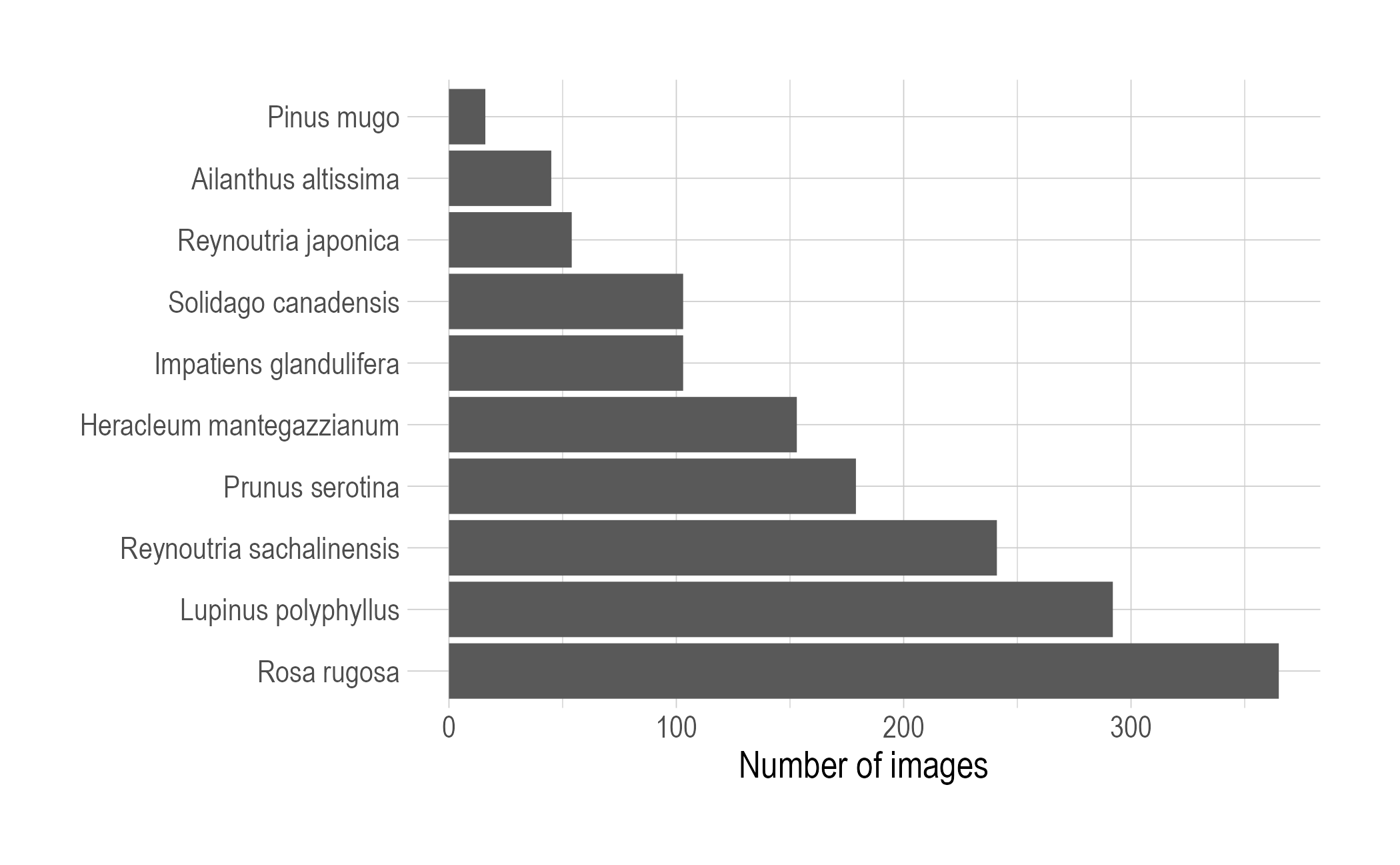
Some of the scores are low even though we’ve picked the highest scoring images for each species in a tagging event. So we could filter by scores to get the number of images down a notch.
library(ggridges)

annotation_samples |>
  ggplot(aes(x = score , y = scientificname)) +
  geom_density_ridges(scale = 2,
                      rel_min_height = 0.01,
                      alpha = 0.7,
                      color = "darkgrey") +
  scale_x_continuous(expand = c(0, 0)) +
  scale_y_discrete(expand = c(0,0)) +
  labs(title = 'Distribution of scores') +
  theme_ridges(font_size = 13, grid = TRUE) +
  theme(axis.title.y = element_blank())
#> Picking joint bandwidth of 0.0453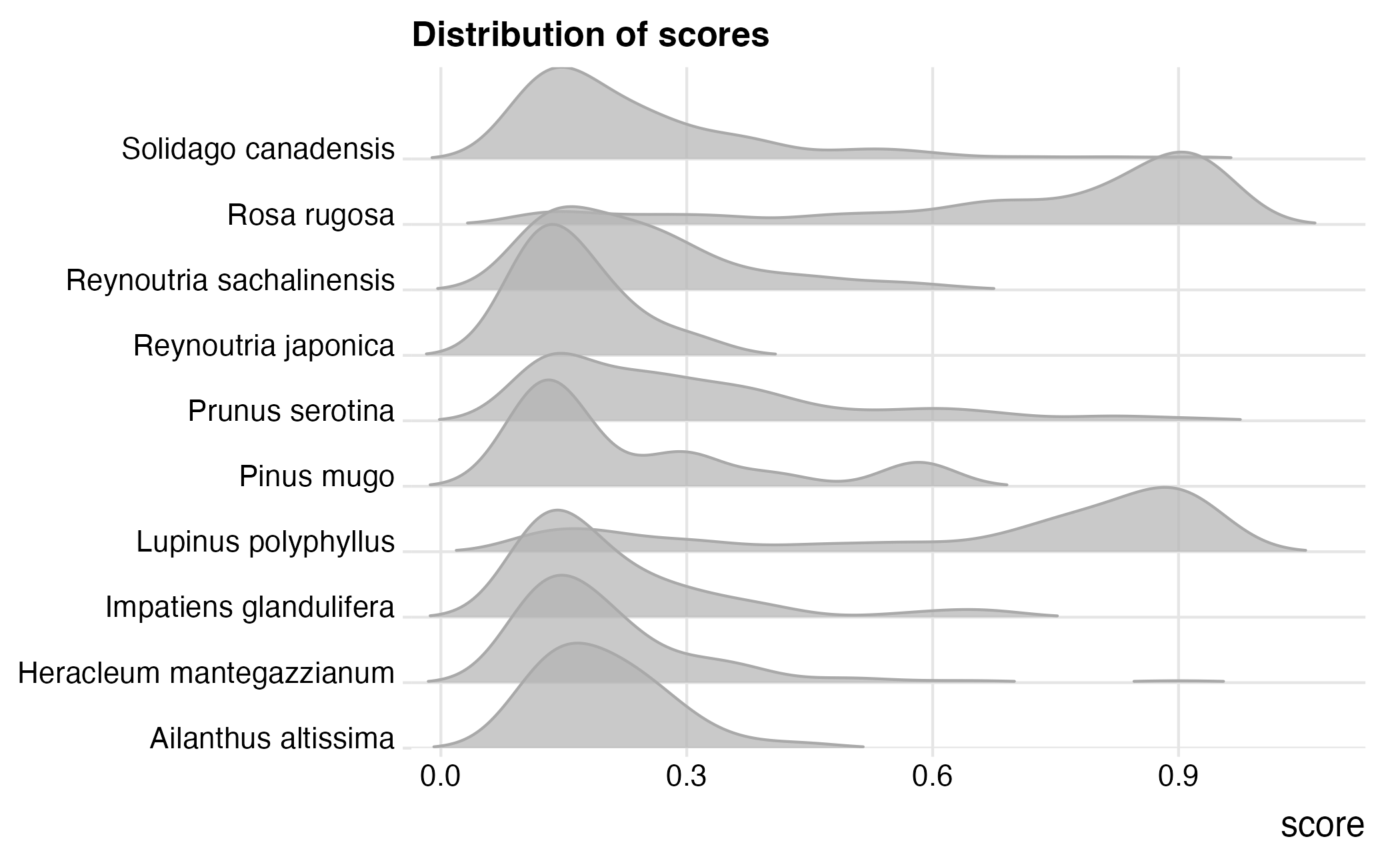
Here take the n highest ranking images for each species.
Adjust n to adjust the number images selected for
annotation..
annotation_samples |>
  group_by(scientificname) |>
  arrange(desc(score), .by_group = TRUE) |>
  slice_head(n = 5) |>
  select(scientificname, imageurl)
#> # A tibble: 50 × 2
#> # Groups:   scientificname [10]
#>    scientificname           imageurl
#>    <chr>                    <chr>
#>  1 Ailanthus altissima      https://anon.erda.au.dk/share_redirect/HO2mESGt0O/r…
#>  2 Ailanthus altissima      https://anon.erda.au.dk/share_redirect/HO2mESGt0O/r…
#>  3 Ailanthus altissima      https://anon.erda.au.dk/share_redirect/HO2mESGt0O/r…
#>  4 Ailanthus altissima      https://anon.erda.au.dk/share_redirect/HO2mESGt0O/r…
#>  5 Ailanthus altissima      https://anon.erda.au.dk/share_redirect/HO2mESGt0O/r…
#>  6 Heracleum mantegazzianum https://anon.erda.au.dk/share_redirect/HO2mESGt0O/r…
#>  7 Heracleum mantegazzianum https://anon.erda.au.dk/share_redirect/HO2mESGt0O/r…
#>  8 Heracleum mantegazzianum https://anon.erda.au.dk/share_redirect/HO2mESGt0O/r…
#>  9 Heracleum mantegazzianum https://anon.erda.au.dk/share_redirect/HO2mESGt0O/r…
#> 10 Heracleum mantegazzianum https://anon.erda.au.dk/share_redirect/HO2mESGt0O/r…
#> # ℹ 40 more rows
  # readr::write_tsv(fs::path_home("Desktop", "camalien-test.tsv"))