Detections

The detections made via the Plantnet API are stored in the detection table. At first we only want to look at the detections for the list of invasive alien species on the “most wanted” list for Denmark. The list of IAS is included in the camalienr package via camalienr::ias. As the same species can be detected in multiple partner countries we also need to filter data to only include data from Denmark in this case.

library(camalienr)
#> camalienr v0.3.6
library(dplyr, warn.conflicts = FALSE)

con <- ca_connect()

ias |> 
  filter(partner == "Denmark") -> ias_dk 
ias_dk_gbifids <- ias_dk$gbifid

con |> 
  ca_get_species() |> 
  filter(gbifid %in% ias_dk_gbifids) |> 
  select(speciesid = pnid, 
         name = scientificname) -> dk_species

dk_join <- ca_get_join_tbl(con, partner_name = "Denmark") |> 
  select(chunkid)

con |> 
  ca_get_image() |> 
  filter(type == "jpg") |>
  select(imageid = id, imagemetaid, chunkid) |> 
  semi_join(dk_join, by = "chunkid") -> dk_images

con |> 
  ca_get_plantnetcall() |> 
  filter(responsestatus == 200) |> 
  select(callid = id, imageid, imageurl, timestamp) |> 
  semi_join(dk_images, by = "imageid") -> dk_calls

con |> 
  ca_get_detection() |> 
  filter(score > 0.3) |> 
  semi_join(dk_calls, by = "callid") |> 
  inner_join(dk_species, by = "speciesid") -> dk_ias
dk_ias
#> # Source:   SQL [?? x 9]
#> # Database: postgres  [au206907@ecos-postgis-prod.cluster-cjqc9gl8vdbe.eu-north-1.rds.amazonaws.com:5432/camalien]
#>         id callid            boxid score boxsize centerx centery speciesid name 
#>    <int64> <chr>             <chr> <dbl>   <int>   <int>   <int>   <int64> <chr>
#>  1 2754904 69c6efb7-07c6-42… e40f… 0.514     384    1184     828   1367432 Lupi…
#>  2 2754914 69c6efb7-07c6-42… d888… 0.386     384    1568     444   1367432 Lupi…
#>  3 2754916 69c6efb7-07c6-42… 144d… 0.390     384    1568    1404   1367432 Lupi…
#>  4 2754923 69c6efb7-07c6-42… 3134… 0.340     384    1760    1596   1367432 Lupi…
#>  5 2754929 69c6efb7-07c6-42… f5b4… 0.568     384    2144     252   1367432 Lupi…
#>  6 2754931 69c6efb7-07c6-42… 7b56… 0.588     384    2336     252   1367432 Lupi…
#>  7 2754935 69c6efb7-07c6-42… ecb1… 0.458     384    2528     252   1367432 Lupi…
#>  8 2754938 69c6efb7-07c6-42… 2993… 0.330     384    2720     252   1367432 Lupi…
#>  9 2754941 69c6efb7-07c6-42… 9a5b… 0.384     384    2912     252   1367432 Lupi…
#> 10 2754943 69c6efb7-07c6-42… 7991… 0.691     384    3104     252   1367432 Lupi…
#> # ℹ more rows

As there can be multiple detections of the same species in an image we need to count the number of images with at least one detection of the species to figure out how many pictures have one of the target species in them. In the detections table we don’t have and id on the image, but we can use the fact that one call is one image.

dk_ias |> 
  summarise(n_imgs = n_distinct(callid), .by = name) |> 
  arrange(desc(n_imgs)) |> 
  collect()
#> # A tibble: 10 × 2
#>    name                      n_imgs
#>    <chr>                    <int64>
#>  1 Lupinus polyphyllus         9121
#>  2 Rosa rugosa                 5194
#>  3 Prunus serotina              268
#>  4 Heracleum mantegazzianum     109
#>  5 Reynoutria sachalinensis      84
#>  6 Solidago canadensis           70
#>  7 Impatiens glandulifera        26
#>  8 Pinus mugo                    25
#>  9 Ailanthus altissima            5
#> 10 Reynoutria japonica            3

Notice that we don’t call collect function until the very end of the pipeline in order to utilize the fact that the database can do the heavy computations for us.

So in the Danish case the detections are heavily biased towards two species.

Performance

Each detection get a score which can be thought of as a probability of the target species being in the image (or part of an image). The distribution of those scores is interesting, so let’s visualize them. Here we use the ggridges package to make ridgeline plots of the scores.

library(ggridges)
library(ggplot2)

ggplot(dk_ias, aes(x = score , y = name)) +
  geom_density_ridges(scale = 2,
                      rel_min_height = 0.01,
                      alpha = 0.7,
                      color = "darkgrey") +
  scale_x_continuous(expand = c(0, 0)) +
  scale_y_discrete(expand = c(0,0)) +
  labs(title = 'Distribution of scores') +
  theme_ridges(font_size = 13, grid = TRUE) + 
  theme(axis.title.y = element_blank())
#> Picking joint bandwidth of 0.0253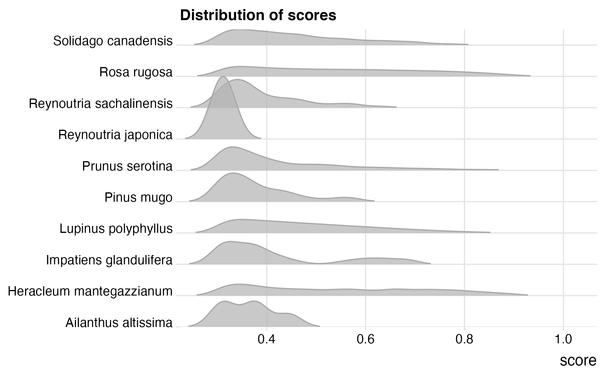

Images

The images as such are not stored on the database, but on the ERDA data warehouse at Aarhus University. The paths to the images in contrast are stored on the database so to view an image we need to find the path (a URL really) to the image and view it some how. The camalienr package provides methods to view images in the viewer in RStudio, but it is possible to simply use a web browser also.

As an example of using the functions in camalienr we look at some of the images where Heracleum mantegazzianum was predicted to be present. To do this we first need to find the image IDs with detections of H. mantegazzianum in the detection table and then find the paths to those images in the plantnetcall table.

dk_ias |> 
  filter(name == "Heracleum mantegazzianum",
         score > 0.3) |> 
  select(callid, boxsize, centerx, centery) |> 
  distinct() -> heracleum

dk_calls |>   
  right_join(heracleum, by = "callid") |> 
  select(callid, starts_with("image"), boxsize, centerx, centery) |>
  collect() -> heracleum_imgs

Right, now we that we have the URLs we can request the image from the ERDA store and view it.

heracleum_imgs$imageurl[1] |>
  ca_img_read() |>
  ca_img_plot(height = 1024L)

This show that we can read an image from the URL and plot it (while scaling to better fit the plotting window). This can be quite handy, but often we would want to see the polygon within which the detection was made. To do this we can pass our heracleum_imgs data.frame to the ca_img_detection() function. This function will read the image from the imageurl column in the data.frame and also plot the polygon that can be constructed from centerx, centery and size.

heracleum_imgs[1,] |>
  ca_img_detection(height = 1024L, border = "red", lwd = 3) 

Positions

Up until now we’ve looked at scores from the image recognition model at Plantnet, we’ve looked at some of the images and located the polygons with detections. We have yet to look at where the species were detected. The position of each image is stored on the database, but there are a few steps we need to take before we can plot a useful map. The outline looks something like this:

1. Find the images with detections of the species of interest
2. Find the positions in the imagemeta table via the imageid column
3. Convert positions to sf
4. Get the URL to the actual images so we can have a nice popup with image taken at the position plotted on the map.
5. Visualize using mapview::mapview()

dk_ias |> 
  filter(name == "Heracleum mantegazzianum", 
         score > 0.3) |> 
  distinct() -> heracleum_imgs

dk_calls |> 
  right_join(heracleum_imgs, by = "callid") |> 
  select(callid, starts_with("image")) -> heracleum_imgs

con |> 
  ca_get_imagemeta() |> 
  filter(velocity > 0) |> 
  select(id, position) -> meta

dk_images |> 
  select(-chunkid) |> 
  right_join(heracleum_imgs, by = "imageid")  |> 
  distinct() |> 
  left_join(meta, by = c("imagemetaid" = "id")) |> 
  collect() -> heracleum_positions

Right, now we have what we need from the database. Now we can convert to sf.

heracleum_positions |> 
  ca_as_sf() -> tmp

And finally let’s see the map. Click on any of the points to see the image that was taken at the location of the point.

mapview::mapview(
  tmp,
  popup = leafpop::popupImage(
    tmp$imageurl,
    src = "remote",
    width = 400 * 1.37,
    height = 400
  ),
  map.types = "OpenStreetMap",
  homebutton = FALSE,
  layer.name = "Heracleum mantegazzianum"
)